
# 第 12 章 pandas 高级应用
前面的章节关注于不同类型的数据规整流程和NumPy、pandas与其它库的特点。随着时间的发展,pandas发展出了更多适合高级用户的功能。本章就要深入学习pandas的高级功能。
# 12.1 分类数据
这一节介绍的是pandas的分类类型。我会向你展示通过使用它,提高性能和内存的使用率。我还会介绍一些在统计和机器学习中使用分类数据的工具。
## 背景和目的
表中的一列通常会有重复的包含不同值的小集合的情况。我们已经学过了unique和value_counts,它们可以从数组提取出不同的值,并分别计算频率:
```python
In [10]: import numpy as np; import pandas as pd
In [11]: values = pd.Series(['apple', 'orange', 'apple',
....: 'apple'] * 2)
In [12]: values
Out[12]:
0 apple
1 orange
2 apple
3 apple
4 apple
5 orange
6 apple
7 apple
dtype: object
In [13]: pd.unique(values)
Out[13]: array(['apple', 'orange'], dtype=object)
In [14]: pd.value_counts(values)
Out[14]:
apple 6
orange 2
dtype: int64
```
许多数据系统(数据仓库、统计计算或其它应用)都发展出了特定的表征重复值的方法,以进行高效的存储和计算。在数据仓库中,最好的方法是使用所谓的包含不同值的维表(Dimension Table),将主要的参数存储为引用维表整数键:
```python
In [15]: values = pd.Series([0, 1, 0, 0] * 2)
In [16]: dim = pd.Series(['apple', 'orange'])
In [17]: values
Out[17]:
0 0
1 1
2 0
3 0
4 0
5 1
6 0
7 0
dtype: int64
In [18]: dim
Out[18]:
0 apple
1 orange
dtype: object
```
可以使用take方法存储原始的字符串Series:
```python
In [19]: dim.take(values)
Out[19]:
0 apple
1 orange
0 apple
0 apple
0 apple
1 orange
0 apple
0 apple
dtype: object
```
这种用整数表示的方法称为分类或字典编码表示法。不同值得数组称为分类、字典或数据级。本书中,我们使用分类的说法。表示分类的整数值称为分类编码或简单地称为编码。
分类表示可以在进行分析时大大的提高性能。你也可以在保持编码不变的情况下,对分类进行转换。一些相对简单的转变例子包括:
- 重命名分类。
- 加入一个新的分类,不改变已经存在的分类的顺序或位置。
## pandas的分类类型
pandas有一个特殊的分类类型,用于保存使用整数分类表示法的数据。看一个之前的Series例子:
```python
In [20]: fruits = ['apple', 'orange', 'apple', 'apple'] * 2
In [21]: N = len(fruits)
In [22]: df = pd.DataFrame({'fruit': fruits,
....: 'basket_id': np.arange(N),
....: 'count': np.random.randint(3, 15, size=N),
....: 'weight': np.random.uniform(0, 4, size=N)},
....: columns=['basket_id', 'fruit', 'count', 'weight'])
In [23]: df
Out[23]:
basket_id fruit count weight
0 0 apple 5 3.858058
1 1 orange 8 2.612708
2 2 apple 4 2.995627
3 3 apple 7 2.614279
4 4 apple 12 2.990859
5 5 orange 8 3.845227
6 6 apple 5 0.033553
7 7 apple 4 0.425778
```
这里,df['fruit']是一个Python字符串对象的数组。我们可以通过调用它,将它转变为分类:
```python
In [24]: fruit_cat = df['fruit'].astype('category')
In [25]: fruit_cat
Out[25]:
0 apple
1 orange
2 apple
3 apple
4 apple
5 orange
6 apple
7 apple
Name: fruit, dtype: category
Categories (2, object): [apple, orange]
```
fruit_cat的值不是NumPy数组,而是一个pandas.Categorical实例:
```python
In [26]: c = fruit_cat.values
In [27]: type(c)
Out[27]: pandas.core.categorical.Categorical
```
分类对象有categories和codes属性:
```python
In [28]: c.categories
Out[28]: Index(['apple', 'orange'], dtype='object')
In [29]: c.codes
Out[29]: array([0, 1, 0, 0, 0, 1, 0, 0], dtype=int8)
```
你可将DataFrame的列通过分配转换结果,转换为分类:
```python
In [30]: df['fruit'] = df['fruit'].astype('category')
In [31]: df.fruit
Out[31]:
0 apple
1 orange
2 apple
3 apple
4 apple
5 orange
6 apple
7 apple
Name: fruit, dtype: category
Categories (2, object): [apple, orange]
```
你还可以从其它Python序列直接创建pandas.Categorical:
```python
In [32]: my_categories = pd.Categorical(['foo', 'bar', 'baz', 'foo', 'bar'])
In [33]: my_categories
Out[33]:
[foo, bar, baz, foo, bar]
Categories (3, object): [bar, baz, foo]
```
如果你已经从其它源获得了分类编码,你还可以使用from_codes构造器:
```python
In [34]: categories = ['foo', 'bar', 'baz']
In [35]: codes = [0, 1, 2, 0, 0, 1]
In [36]: my_cats_2 = pd.Categorical.from_codes(codes, categories)
In [37]: my_cats_2
Out[37]:
[foo, bar, baz, foo, foo, bar]
Categories (3, object): [foo, bar, baz]
```
与显示指定不同,分类变换不认定指定的分类顺序。因此取决于输入数据的顺序,categories数组的顺序会不同。当使用from_codes或其它的构造器时,你可以指定分类一个有意义的顺序:
```python
In [38]: ordered_cat = pd.Categorical.from_codes(codes, categories,
....: ordered=True)
In [39]: ordered_cat
Out[39]:
[foo, bar, baz, foo, foo, bar]
Categories (3, object): [foo < bar < baz]
```
输出[foo < bar < baz]指明‘foo’位于‘bar’的前面,以此类推。无序的分类实例可以通过as_ordered排序:
```python
In [40]: my_cats_2.as_ordered()
Out[40]:
[foo, bar, baz, foo, foo, bar]
Categories (3, object): [foo < bar < baz]
```
最后要注意,分类数据不需要字符串,尽管我仅仅展示了字符串的例子。分类数组可以包括任意不可变类型。
## 用分类进行计算
与非编码版本(比如字符串数组)相比,使用pandas的Categorical有些类似。某些pandas组件,比如groupby函数,更适合进行分类。还有一些函数可以使用有序标志位。
来看一些随机的数值数据,使用pandas.qcut面元函数。它会返回pandas.Categorical,我们之前使用过pandas.cut,但没解释分类是如何工作的:
```python
In [41]: np.random.seed(12345)
In [42]: draws = np.random.randn(1000)
In [43]: draws[:5]
Out[43]: array([-0.2047, 0.4789, -0.5194, -0.5557, 1.9658])
```
计算这个数据的分位面元,提取一些统计信息:
```python
In [44]: bins = pd.qcut(draws, 4)
In [45]: bins
Out[45]:
[(-0.684, -0.0101], (-0.0101, 0.63], (-0.684, -0.0101], (-0.684, -0.0101], (0.63,
3.928], ..., (-0.0101, 0.63], (-0.684, -0.0101], (-2.95, -0.684], (-0.0101, 0.63
], (0.63, 3.928]]
Length: 1000
Categories (4, interval[float64]): [(-2.95, -0.684] < (-0.684, -0.0101] < (-0.010
1, 0.63] <
(0.63, 3.928]]
```
虽然有用,确切的样本分位数与分位的名称相比,不利于生成汇总。我们可以使用labels参数qcut,实现目的:
```python
In [46]: bins = pd.qcut(draws, 4, labels=['Q1', 'Q2', 'Q3', 'Q4'])
In [47]: bins
Out[47]:
[Q2, Q3, Q2, Q2, Q4, ..., Q3, Q2, Q1, Q3, Q4]
Length: 1000
Categories (4, object): [Q1 < Q2 < Q3 < Q4]
In [48]: bins.codes[:10]
Out[48]: array([1, 2, 1, 1, 3, 3, 2, 2, 3, 3], dtype=int8)
```
加上标签的面元分类不包含数据面元边界的信息,因此可以使用groupby提取一些汇总信息:
```python
In [49]: bins = pd.Series(bins, name='quartile')
In [50]: results = (pd.Series(draws)
....: .groupby(bins)
....: .agg(['count', 'min', 'max'])
....: .reset_index())
In [51]: results
Out[51]:
quartile count min max
0 Q1 250 -2.949343 -0.685484
1 Q2 250 -0.683066 -0.010115
2 Q3 250 -0.010032 0.628894
3 Q4 250 0.634238 3.927528
```
分位数列保存了原始的面元分类信息,包括排序:
```python
In [52]: results['quartile']
Out[52]:
0 Q1
1 Q2
2 Q3
3 Q4
Name: quartile, dtype: category
Categories (4, object): [Q1 < Q2 < Q3 < Q4]
```
## 用分类提高性能
如果你是在一个特定数据集上做大量分析,将其转换为分类可以极大地提高效率。DataFrame列的分类使用的内存通常少的多。来看一些包含一千万元素的Series,和一些不同的分类:
```python
In [53]: N = 10000000
In [54]: draws = pd.Series(np.random.randn(N))
In [55]: labels = pd.Series(['foo', 'bar', 'baz', 'qux'] * (N // 4))
```
现在,将标签转换为分类:
```python
In [56]: categories = labels.astype('category')
```
这时,可以看到标签使用的内存远比分类多:
```python
In [57]: labels.memory_usage()
Out[57]: 80000080
In [58]: categories.memory_usage()
Out[58]: 10000272
```
转换为分类不是没有代价的,但这是一次性的代价:
```python
In [59]: %time _ = labels.astype('category')
CPU times: user 490 ms, sys: 240 ms, total: 730 ms
Wall time: 726 ms
```
GroupBy使用分类操作明显更快,是因为底层的算法使用整数编码数组,而不是字符串数组。
## 分类方法
包含分类数据的Series有一些特殊的方法,类似于Series.str字符串方法。它还提供了方便的分类和编码的使用方法。看下面的Series:
```python
In [60]: s = pd.Series(['a', 'b', 'c', 'd'] * 2)
In [61]: cat_s = s.astype('category')
In [62]: cat_s
Out[62]:
0 a
1 b
2 c
3 d
4 a
5 b
6 c
7 d
dtype: category
Categories (4, object): [a, b, c, d]
```
特别的cat属性提供了分类方法的入口:
```python
In [63]: cat_s.cat.codes
Out[63]:
0 0
1 1
2 2
3 3
4 0
5 1
6 2
7 3
dtype: int8
In [64]: cat_s.cat.categories
Out[64]: Index(['a', 'b', 'c', 'd'], dtype='object')
```
假设我们知道这个数据的实际分类集,超出了数据中的四个值。我们可以使用set_categories方法改变它们:
```python
In [65]: actual_categories = ['a', 'b', 'c', 'd', 'e']
In [66]: cat_s2 = cat_s.cat.set_categories(actual_categories)
In [67]: cat_s2
Out[67]:
0 a
1 b
2 c
3 d
4 a
5 b
6 c
7 d
dtype: category
Categories (5, object): [a, b, c, d, e]
```
虽然数据看起来没变,新的分类将反映在它们的操作中。例如,如果有的话,value_counts表示分类:
```python
In [68]: cat_s.value_counts()
Out[68]:
d 2
c 2
b 2
a 2
dtype: int64
In [69]: cat_s2.value_counts()
Out[69]:
d 2
c 2
b 2
a 2
e 0
dtype: int64
```
在大数据集中,分类经常作为节省内存和高性能的便捷工具。过滤完大DataFrame或Series之后,许多分类可能不会出现在数据中。我们可以使用remove_unused_categories方法删除没看到的分类:
```python
In [70]: cat_s3 = cat_s[cat_s.isin(['a', 'b'])]
In [71]: cat_s3
Out[71]:
0 a
1 b
4 a
5 b
dtype: category
Categories (4, object): [a, b, c, d]
In [72]: cat_s3.cat.remove_unused_categories()
Out[72]:
0 a
1 b
4 a
5 b
dtype: category
Categories (2, object): [a, b]
```
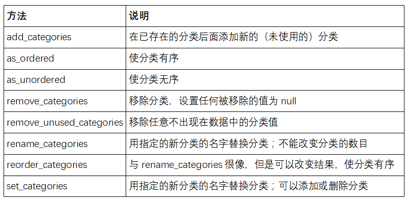
表12-1列出了可用的分类方法。
## 为建模创建虚拟变量
当你使用统计或机器学习工具时,通常会将分类数据转换为虚拟变量,也称为one-hot编码。这包括创建一个不同类别的列的DataFrame;这些列包含给定分类的1s,其它为0。
看前面的例子:
```python
In [73]: cat_s = pd.Series(['a', 'b', 'c', 'd'] * 2, dtype='category')
```
前面的第7章提到过,pandas.get_dummies函数可以转换这个分类数据为包含虚拟变量的DataFrame:
```python
In [74]: pd.get_dummies(cat_s)
Out[74]:
a b c d
0 1 0 0 0
1 0 1 0 0
2 0 0 1 0
3 0 0 0 1
4 1 0 0 0
5 0 1 0 0
6 0 0 1 0
7 0 0 0 1
```
# 12.2 GroupBy高级应用
尽管我们在第10章已经深度学习了Series和DataFrame的Groupby方法,还有一些方法也是很有用的。
## 分组转换和“解封”GroupBy
在第10章,我们在分组操作中学习了apply方法,进行转换。还有另一个transform方法,它与apply很像,但是对使用的函数有一定限制:
- 它可以产生向分组形状广播标量值
- 它可以产生一个和输入组形状相同的对象
- 它不能修改输入
来看一个简单的例子:
```python
In [75]: df = pd.DataFrame({'key': ['a', 'b', 'c'] * 4,
....: 'value': np.arange(12.)})
In [76]: df
Out[76]:
key value
0 a 0.0
1 b 1.0
2 c 2.0
3 a 3.0
4 b 4.0
5 c 5.0
6 a 6.0
7 b 7.0
8 c 8.0
9 a 9.0
10 b 10.0
11 c 11.0
```
按键进行分组:
```python
In [77]: g = df.groupby('key').value
In [78]: g.mean()
Out[78]:
key
a 4.5
b 5.5
c 6.5
Name: value, dtype: float64
```
假设我们想产生一个和df['value']形状相同的Series,但值替换为按键分组的平均值。我们可以传递函数lambda x: x.mean()进行转换:
```python
In [79]: g.transform(lambda x: x.mean())
Out[79]:
0 4.5
1 5.5
2 6.5
3 4.5
4 5.5
5 6.5
6 4.5
7 5.5
8 6.5
9 4.5
10 5.5
11 6.5
Name: value, dtype: float64
```
对于内置的聚合函数,我们可以传递一个字符串假名作为GroupBy的agg方法:
```python
In [80]: g.transform('mean')
Out[80]:
0 4.5
1 5.5
2 6.5
3 4.5
4 5.5
5 6.5
6 4.5
7 5.5
8 6.5
9 4.5
10 5.5
11 6.5
Name: value, dtype: float64
```
与apply类似,transform的函数会返回Series,但是结果必须与输入大小相同。举个例子,我们可以用lambda函数将每个分组乘以2:
```python
In [81]: g.transform(lambda x: x * 2)
Out[81]:
0 0.0
1 2.0
2 4.0
3 6.0
4 8.0
5 10.0
6 12.0
7 14.0
8 16.0
9 18.0
10 20.0
11 22.0
Name: value, dtype: float64
```
再举一个复杂的例子,我们可以计算每个分组的降序排名:
```python
In [82]: g.transform(lambda x: x.rank(ascending=False))
Out[82]:
0 4.0
1 4.0
2 4.0
3 3.0
4 3.0
5 3.0
6 2.0
7 2.0
8 2.0
9 1.0
10 1.0
11 1.0
Name: value, dtype: float64
```
看一个由简单聚合构造的的分组转换函数:
```python
def normalize(x):
return (x - x.mean()) / x.std()
```
我们用transform或apply可以获得等价的结果:
```python
In [84]: g.transform(normalize)
Out[84]:
0 -1.161895
1 -1.161895
2 -1.161895
3 -0.387298
4 -0.387298
5 -0.387298
6 0.387298
7 0.387298
8 0.387298
9 1.161895
10 1.161895
11 1.161895
Name: value, dtype: float64
In [85]: g.apply(normalize)
Out[85]:
0 -1.161895
1 -1.161895
2 -1.161895
3 -0.387298
4 -0.387298
5 -0.387298
6 0.387298
7 0.387298
8 0.387298
9 1.161895
10 1.161895
11 1.161895
Name: value, dtype: float64
```
内置的聚合函数,比如mean或sum,通常比apply函数快,也比transform快。这允许我们进行一个所谓的解封(unwrapped)分组操作:
```python
In [86]: g.transform('mean')
Out[86]:
0 4.5
1 5.5
2 6.5
3 4.5
4 5.5
5 6.5
6 4.5
7 5.5
8 6.5
9 4.5
10 5.5
11 6.5
Name: value, dtype: float64
In [87]: normalized = (df['value'] - g.transform('mean')) / g.transform('std')
In [88]: normalized
Out[88]:
0 -1.161895
1 -1.161895
2 -1.161895
3 -0.387298
4 -0.387298
5 -0.387298
6 0.387298
7 0.387298
8 0.387298
9 1.161895
10 1.161895
11 1.161895
Name: value, dtype: float64
```
解封分组操作可能包括多个分组聚合,但是矢量化操作还是会带来收益。
## 分组的时间重采样
对于时间序列数据,resample方法从语义上是一个基于内在时间的分组操作。下面是一个示例表:
```python
In [89]: N = 15
In [90]: times = pd.date_range('2017-05-20 00:00', freq='1min', periods=N)
In [91]: df = pd.DataFrame({'time': times,
....: 'value': np.arange(N)})
In [92]: df
Out[92]:
time value
0 2017-05-20 00:00:00 0
1 2017-05-20 00:01:00 1
2 2017-05-20 00:02:00 2
3 2017-05-20 00:03:00 3
4 2017-05-20 00:04:00 4
5 2017-05-20 00:05:00 5
6 2017-05-20 00:06:00 6
7 2017-05-20 00:07:00 7
8 2017-05-20 00:08:00 8
9 2017-05-20 00:09:00 9
10 2017-05-20 00:10:00 10
11 2017-05-20 00:11:00 11
12 2017-05-20 00:12:00 12
13 2017-05-20 00:13:00 13
14 2017-05-20 00:14:00 14
```
这里,我们可以用time作为索引,然后重采样:
```python
In [93]: df.set_index('time').resample('5min').count()
Out[93]:
value
time
2017-05-20 00:00:00 5
2017-05-20 00:05:00 5
2017-05-20 00:10:00 5
```
假设DataFrame包含多个时间序列,用一个额外的分组键的列进行标记:
```python
In [94]: df2 = pd.DataFrame({'time': times.repeat(3),
....: 'key': np.tile(['a', 'b', 'c'], N),
....: 'value': np.arange(N * 3.)})
In [95]: df2[:7]
Out[95]:
key time value
0 a 2017-05-20 00:00:00 0.0
1 b 2017-05-20 00:00:00 1.0
2 c 2017-05-20 00:00:00 2.0
3 a 2017-05-20 00:01:00 3.0
4 b 2017-05-20 00:01:00 4.0
5 c 2017-05-20 00:01:00 5.0
6 a 2017-05-20 00:02:00 6.0
```
要对每个key值进行相同的重采样,我们引入pandas.TimeGrouper对象:
```python
In [96]: time_key = pd.TimeGrouper('5min')
```
我们然后设定时间索引,用key和time_key分组,然后聚合:
```python
In [97]: resampled = (df2.set_index('time')
....: .groupby(['key', time_key])
....: .sum())
In [98]: resampled
Out[98]:
value
key time
a 2017-05-20 00:00:00 30.0
2017-05-20 00:05:00 105.0
2017-05-20 00:10:00 180.0
b 2017-05-20 00:00:00 35.0
2017-05-20 00:05:00 110.0
2017-05-20 00:10:00 185.0
c 2017-05-20 00:00:00 40.0
2017-05-20 00:05:00 115.0
2017-05-20 00:10:00 190.0
In [99]: resampled.reset_index()
Out[99]:
key time value
0 a 2017-05-20 00:00:00 30.0
1 a 2017-05-20 00:05:00 105.0
2 a 2017-05-20 00:10:00 180.0
3 b 2017-05-20 00:00:00 35.0
4 b 2017-05-20 00:05:00 110.0
5 b 2017-05-20 00:10:00 185.0
6 c 2017-05-20 00:00:00 40.0
7 c 2017-05-20 00:05:00 115.0
8 c 2017-05-20 00:10:00 190.0
```
使用TimeGrouper的限制是时间必须是Series或DataFrame的索引。
# 12.3 链式编程技术
当对数据集进行一系列变换时,你可能发现创建的多个临时变量其实并没有在分析中用到。看下面的例子:
```python
df = load_data()
df2 = df[df['col2'] < 0]
df2['col1_demeaned'] = df2['col1'] - df2['col1'].mean()
result = df2.groupby('key').col1_demeaned.std()
```
虽然这里没有使用真实的数据,这个例子却指出了一些新方法。首先,DataFrame.assign方法是一个df[k] = v形式的函数式的列分配方法。它不是就地修改对象,而是返回新的修改过的DataFrame。因此,下面的语句是等价的:
```python
# Usual non-functional way
df2 = df.copy()
df2['k'] = v
# Functional assign way
df2 = df.assign(k=v)
```
就地分配可能会比assign快,但是assign可以方便地进行链式编程:
```python
result = (df2.assign(col1_demeaned=df2.col1 - df2.col2.mean())
.groupby('key')
.col1_demeaned.std())
```
我使用外括号,这样便于添加换行符。
使用链式编程时要注意,你可能会需要涉及临时对象。在前面的例子中,我们不能使用load_data的结果,直到它被赋值给临时变量df。为了这么做,assign和许多其它pandas函数可以接收类似函数的参数,即可调用对象(callable)。为了展示可调用对象,看一个前面例子的片段:
```python
df = load_data()
df2 = df[df['col2'] < 0]
```
它可以重写为:
```python
df = (load_data()
[lambda x: x['col2'] < 0])
```
这里,load_data的结果没有赋值给某个变量,因此传递到[ ]的函数在这一步被绑定到了对象。
我们可以把整个过程写为一个单链表达式:
```python
result = (load_data()
[lambda x: x.col2 < 0]
.assign(col1_demeaned=lambda x: x.col1 - x.col1.mean())
.groupby('key')
.col1_demeaned.std())
```
是否将代码写成这种形式只是习惯而已,将它分开成若干步可以提高可读性。
## 管道方法
你可以用Python内置的pandas函数和方法,用带有可调用对象的链式编程做许多工作。但是,有时你需要使用自己的函数,或是第三方库的函数。这时就要用到管道方法。
看下面的函数调用:
```python
a = f(df, arg1=v1)
b = g(a, v2, arg3=v3)
c = h(b, arg4=v4)
```
当使用接收、返回Series或DataFrame对象的函数式,你可以调用pipe将其重写:
```python
result = (df.pipe(f, arg1=v1)
.pipe(g, v2, arg3=v3)
.pipe(h, arg4=v4))
```
f(df)和df.pipe(f)是等价的,但是pipe使得链式声明更容易。
pipe的另一个有用的地方是提炼操作为可复用的函数。看一个从列减去分组方法的例子:
```python
g = df.groupby(['key1', 'key2'])
df['col1'] = df['col1'] - g.transform('mean')
```
假设你想转换多列,并修改分组的键。另外,你想用链式编程做这个转换。下面就是一个方法:
```python
def group_demean(df, by, cols):
result = df.copy()
g = df.groupby(by)
for c in cols:
result[c] = df[c] - g[c].transform('mean')
return result
```
然后可以写为:
```python
result = (df[df.col1 < 0]
.pipe(group_demean, ['key1', 'key2'], ['col1']))
```
# 12.4 总结
和其它许多开源项目一样,pandas仍然在不断的变化和进步中。和本书中其它地方一样,这里的重点是放在接下来几年不会发生什么改变且稳定的功能。
为了深入学习pandas的知识,我建议你学习官方文档,并阅读开发团队发布的文档更新。我们还邀请你加入pandas的开发工作:修改bug、创建新功能、完善文档。
- 利用 Python 进行数据分析 · 第 2 版
- 第 1 章 准备工作
- 第 2 章 Python 语法基础,IPython 和 Jupyter Notebooks
- 第 3 章 Python 的数据结构、函数和文件
- 第 4 章 NumPy 基础:数组和矢量计算
- 第 5 章 pandas 入门
- 第 6 章 数据加载、存储与文件格式
- 第 7 章 数据清洗和准备
- 第 8 章 数据规整:聚合、合并和重塑
- 第 9 章 绘图和可视化
- 第 10 章 数据聚合与分组运算
- 第 11 章 时间序列
- 第 12 章 pandas 高级应用
- 第 13 章 Python 建模库介绍
- 第 14 章 数据分析案例
- 附录 A NumPy 高级应用
- 附录 B 更多关于 IPython 的内容